The t-test is a foundational statistical hypothesis test used to determine if there is a significant difference between the means of two groups, which may be related in certain features.
It is applied when the test statistic follows a normal distribution and the value of a scaling term in the test statistic follows a Student’s t-distribution under the null hypothesis.
The t-test is most commonly applied when the test statistic would follow a normal distribution if the value of a scaling term in the test statistic were known. When the scaling term is unknown and is replaced by an estimate based on the data, the test statistics (under certain conditions) follow a Student’s t distribution.
When to use T test
Small Samples: The T-test extends the principles learned from the Z-test to situations where the sample size is small (usually n < 30) and the population variance is unknown. It introduces the concept of using sample data to estimate population parameters, adding a layer of complexity.
Student’s T-Distribution: The T-test introduces a new distribution, the T-distribution, which is more spread out than the Z-distribution, especially for small sample sizes. The shape of the T-distribution changes with the degrees of freedom, a concept not encountered with the Z-distribution.
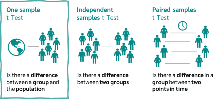
Types of T-Tests
There are three main types of t-tests, each suited for different testing scenarios:
One-sample t-test: This test compares the mean of a single group against a known standard or mean. For instance, it could be used to determine if the average process time for completing a task is different from the standard time.
Independent Samples t-test: This test compares the means of two independent groups in order to determine whether there is statistical evidence that the associated population means are significantly different. It is used when the variances of two normal distributions are unknown and the samples are independent. A common example is comparing the test scores of two different groups of students.
Paired Samples t-test: This test is used to compare the means of the same group or related samples at two different points in time or under two different conditions. It’s often used in before-and-after studies, such as measuring the effect of a training program on the performance of athletes by measuring them before and after the program.
source: https://datatab.net/tutorial/one-sample-t-test
Applications
The t-test has widespread applications across various fields such as:
-
Education: To compare test scores, teaching methods, or learning outcomes.
-
Medicine: For assessing the effectiveness of treatments or drugs.
-
Manufacturing and quality control: To determine if the process changes have led to improvements.
-
Social sciences: To compare differences in social, psychological, or behavioral effects across groups.
Assumptions
For the t-test to be valid, certain assumptions must be met:
-
Independence of Observations: Each observation must be independent of all other observations.
-
Normality: The data should be approximately normally distributed, especially as the sample size increases (Central Limit Theorem).
-
Equality of Variances (for independent samples t-test): The variances of the two groups being compared should be equal. When this assumption is violated, a variation of the t-test called Welch’s t-test can be used.
Interpretation
The output of a t-test is a p-value, which indicates the probability of observing the test results under the null hypothesis. If the p-value is below a predetermined threshold (commonly 0.05), the null hypothesis is rejected, indicating that there is a statistically significant difference between the groups being compared.
The t-test is a robust tool with wide applicability but must be used judiciously, respecting its assumptions for valid results. Advances in statistical methodologies have introduced more complex models for data analysis, yet the t-test remains a fundamental and widely used method for comparing means.
Concept of Degrees of Freedom in T-Tests
Degrees of freedom (df) in statistics generally refer to the number of values in a calculation that are free to vary without violating any constraints.
In the context of a t-test, degrees of freedom are crucial for determining the specific distribution of the t-statistic under the null hypothesis.
- A t-test is used to determine if there is a significant difference between the means of two groups under the assumption that the data follows a normal distribution but when the population standard deviation is not known.
- The t-test uses the sample standard deviation as an estimate of the population standard deviation. This estimation introduces more variability and uncertainty, which is why the t-distribution, rather than the normal distribution, is used.
- The t-distribution is wider and has thicker tails than the normal distribution, which accounts for this additional uncertainty.
Degrees of freedom in different types of t-tests:
One-Sample t-test:
df = n - 1, where \(n\) is the number of observations in the sample. Subtracting one accounts for the estimation of the sample mean from the sample data itself.
Independent Two-Sample t-test:
df = \(n_1\) + \(n_2\) - 2, where \(n_1\) and \(n_2\) are the sample sizes of the two groups. Here, two degrees are lost because each group’s mean is estimated from its sample.
Paired t-test:
df = n - 1. In paired samples, each pair’s difference is considered as a single piece of data. If there are \(n\) pairs, the degrees of freedom are n - 1, reflecting the \(n\) paired differences.
Why Z-Tests don’t have Degrees of Freedom 🤔 ?
The Z-test, unlike the t-test, does not involve degrees of freedom because it uses the population standard deviation (\(\sigma\)), which is assumed to be known.
Because the Z-test uses the actual population standard deviation and not an estimate from the sample, there is no extra uncertainty introduced by estimation that needs to be accounted for using degrees of freedom.
Consequently, the distribution of the Z-test statistic under the null hypothesis is the standard normal distribution (Z-distribution), which is not dependent on the sample size once the population standard deviation is known.
One-Sample T-Test
The one-sample t-test is a statistical procedure used to determine whether the mean of a single sample differs significantly from a known or hypothesized population mean. This test is particularly useful when the population standard deviation is unknown and the sample size is small, which is a common scenario in many practical research applications.
Assumptions
Before conducting a one-sample t-test, certain assumptions must be verified to ensure the validity of the test results:
-
Normality: The data should be approximately normally distributed. This assumption is especially important with smaller sample sizes. For larger samples, the Central Limit Theorem helps as it suggests that the means of the samples will be approximately normally distributed regardless of the shape of the population distribution.
-
Independence: The sampled observations must be independent of each other. This means that the selection of one observation does not influence or alter the selection of other observations.
-
Scale of Measurement: The data should be measured at least at the interval level, which means that the numerical distances between measurements are defined.
Hypotheses
The hypotheses for a one-sample t-test are structured as follows:
-
Null Hypothesis (H₀): The population mean is equal to the specified value (\(\mu = \mu_0\)).
-
Alternative Hypothesis (H₁): The population mean is not equal to the specified value (\(\mu \neq \mu_0\)). The alternative hypothesis can also be directional, stating that the mean is greater than (\(\mu > \mu_0\)) or less than (\(\mu < \mu_0\)) the specified value, depending on the research question.
Calculating Degrees of Freedom
The degrees of freedom for the one-sample t-test are calculated as \(n - 1\). This value is crucial for determining the critical values from the t-distribution, which are needed to assess the significance of the test statistic.
Interpretation
To decide whether to reject the null hypothesis, compare the calculated t-value to the critical t-value from the t-distribution at the desired significance level (\(\alpha\), often 0.05 for a 5% significance level). The decision rules are:
- If the absolute value of the calculated t-value is greater than the critical t-value, reject the null hypothesis.
- If the absolute value of the calculated t-value is less than or equal to the critical t-value, do not reject the null hypothesis.
One-Sample T-Test Example problem
A bakery claims that its chocolate chip cookies weigh at least 60 grams on average. A quality control manager is skeptical of this claim and decides to test it. She randomly selects 15 cookies and finds the following weights in grams:
52, 55, 61, 54, 58, 59, 62, 53, 56, 57, 60, 59, 61, 64, 58
She decides to use a one-sample t-test to see if there’s evidence that the average weight is different from the bakery’s claim. She chooses a significance level of 0.05.
Hypotheses
- Null Hypothesis (\(H_0\)): \(\mu = 60\) grams. The average weight of the cookies is 60 grams.
- Alternative Hypothesis (\(H_1\)): \(\mu \neq 60\) grams. The average weight of the cookies is not 60 grams.
First, let’s calculate the sample mean (\(\bar{x}\)), sample standard deviation (\(s\)), and the t-statistic.
Calculate the Sample Mean (\(\bar{x}\)):
The sample size \(n\) is 15.
Sample mean = \[
\bar{x} = \frac{\sum \text{sample values}}{n}
\]
\[
= \frac{52 + 55 + 61 + 54 + 58 + 59 + 62 + 53 + 56 + 57 + 60 + 59 + 61 + 64 + 58}{15}
\]
\[
= \frac{866}{15} = 57.73 \text{ grams}
\]
Calculate the Sample Standard Deviation (s):
To calculate \(s\), use the formula:
\[
s = \sqrt{\frac{\sum (x_i - \bar{x})^2}{n-1}}
\]
First, compute the deviations from the mean, square each, and then sum them up:
- \((52 - 57.73)^2 = 32.6729\)
- \((55 - 57.73)^2 = 7.4929\)
- \((61 - 57.73)^2 = 10.6329\)
- \((54 - 57.73)^2 = 13.9129\)
- \((58 - 57.73)^2 = 0.0729\)
- \((59 - 57.73)^2 = 1.6129\)
- \((62 - 57.73)^2 = 18.1929\)
- \((53 - 57.73)^2 = 22.3729\)
- \((56 - 57.73)^2 = 2.9929\)
- \((57 - 57.73)^2 = 0.5329\)
- \((60 - 57.73)^2 = 5.1129\)
- \((59 - 57.73)^2 = 1.6129\)
- \((61 - 57.73)^2 = 10.6329\)
- \((64 - 57.73)^2 = 39.3129\)
- \((58 - 57.73)^2 = 0.0729\)
Sum of squared deviations:
\[
\sum (x_i - \bar{x})^2 = 167.1204
\]
Now calculate \(s\):
\[
s = \sqrt{\frac{167.1204}{14}} = 3.46 \text{ grams}
\]
Compute the T-Statistic:
Using the t-test formula:
\[
t = \frac{\bar{x} - \mu}{s / \sqrt{n}} = \frac{57.73 - 60}{3.46 / \sqrt{15}} = -2.32
\]
Determine Degrees of Freedom:
\[
df = n - 1 = 15 - 1 = 14
\]
Calculate P-Value for a Two-Tailed Test:
Based on the t-statistic, look up or compute the p-value for \(|t| = 2.32\) with \(df = 14\). This value is approximately \(p = 0.036\).
Interpretation
T-Statistic: The negative value of the t-statistic (-2.32) indicates that the sample mean is less than the null hypothesis mean of 60 grams.
P-Value: The p-value of 0.036 is less than the chosen significance level of 0.05. This suggests that there is statistically significant evidence to reject the null hypothesis.
Therefore, based on the sample of 15 cookies, there is sufficient statistical evidence to conclude that the average weight of the bakery’s chocolate chip cookies is different from the claimed 60 grams.
Given the direction indicated by the t-statistic, it suggests that the cookies may, on average, weigh less than the claimed 60 grams.
One-Sample T-Test calculation using Excel:
Download the Excel file link here
One-Sample T-Test calculation using R:
Code
# Sample data
weights <- c(52, 55, 61, 54, 58, 59, 62, 53, 56, 57, 60, 59, 61, 64, 58)
alpha = 0.05
# Calculate sample size
sample_size <- length(weights)
sample_size
Code
# Calculate sample mean
sample_mean <- mean(weights)
sample_mean
Code
# Calculate sample standard deviation (R uses n-1 by default)
sample_sd <- sd(weights)
sample_sd
Code
# Define population mean for comparison
population_mean <- 60
population_mean
Code
# Calculate the t-statistic
t_statistic <- (sample_mean - population_mean) / (sample_sd / sqrt(sample_size))
t_statistic
Code
# Degrees of freedom
degrees_of_freedom <- sample_size - 1
degrees_of_freedom
Code
# Calculate the p-value for a two-tailed test
p_value <- 2 * pt(-abs(t_statistic), df = degrees_of_freedom)
p_value
Code
# Decision based on p-value
if (p_value < alpha) {
  cat("Reject null hypothesis\n")
} else {
  cat("Do not reject null hypothesis\n")
}
One-Sample T-Test calculation using python:
Code
import numpy as np
from scipy import stats
# Sample data
weights = np.array([52, 55, 61, 54, 58, 59, 62, 53, 56, 57, 60, 59, 61, 64, 58])
alpha = 0.05
# Population mean
population_mean = 60

# Sample size
sample_size = len(weights)
sample_size
Code
# Sample mean
sample_mean = np.mean(weights)
sample_mean
Code
# Sample standard deviation
sample_sd = np.std(weights, ddof=1)
sample_sd
Code
# Calculate the t-statistic
t_statistic = (sample_mean - population_mean) / (sample_sd / np.sqrt(sample_size))
t_statistic
Code
# Degrees of freedom
degrees_of_freedom = sample_size - 1
degrees_of_freedom
Code
# Calculate the p-value (two-tailed test)
p_value = 2* stats.t.sf(np.abs(t_statistic), df=degrees_of_freedom)
p_value
Code
# Hypothesis decision
if p_value < alpha:
    print("Reject null hypothesis")
else:
    print("Do not reject null hypothesis")
Independent samples t-test / Two Sample t-test
The independent samples t-test, also known as the two-sample t-test or Student’s t-test, is a statistical procedure used to determine if there is a significant difference between the means of two independent groups. This test is commonly used in situations where you want to compare the means from two different groups, such as two different treatments or conditions, to see if they differ from each other in a statistically significant way.
Assumptions
You would use an independent samples t-test under the following conditions:
-
Independence of Samples: The two groups being compared must be independent, meaning the samples drawn from one group do not influence the samples from the other group.
-
Normally Distributed Data: The data in the two groups should be roughly normally distributed.
-
Equality of Variances: The variances of the two groups are assumed to be equal. If this assumption is significantly violated, a variation of the t-test, like Welch’s t-test, may be used instead.
Hypotheses
The hypotheses for an independent samples t-test are usually framed as follows:
-
Null Hypothesis (H₀): The means of the two groups are equal (\(\mu_1 = \mu_2\)).
-
Alternative Hypothesis (H₁): The means of the two groups are not equal (\(\mu_1 \neq \mu_2\)), which can be two-tailed, or one-tailed if the direction of the difference is specified.
Calculating Degrees of Freedom
The degrees of freedom used in this table are \(n_1 + n_2 - 2\).
Interpretation
To decide whether to reject the null hypothesis, compare the calculated t-value to the critical t-value from the t-distribution at the desired significance level (\(\alpha\), often 0.05 for a 5% significance level). The decision rules are:
- If the absolute value of the calculated t-value is greater than the critical t-value, reject the null hypothesis.
- If the absolute value of the calculated t-value is less than or equal to the critical t-value, do not reject the null hypothesis.
This test allows researchers to understand whether different conditions have a statistically significant impact on the means of the groups being compared, providing crucial insights in fields such as medicine, psychology, and economics.
Two Samples T-Test Example problem
Suppose we want to determine if there is a significant difference in the average test scores between two classes. Class A has 5 students, and Class B has 5 students. Here are their test scores:
-
Class A: 85, 88, 90, 95, 78
-
Class B: 80, 83, 79, 92, 87
Hypotheses:
-
Null Hypothesis (H₀): \(\mu_1 = \mu_2\) (The means of both classes are equal)
-
Alternative Hypothesis (H₁): \(\mu_1 \neq \mu_2\) (The means of both classes are not equal)
We will use a significance level (\(\alpha\)) of 0.05.
To illustrate the mathematics behind the calculations performed for the independent samples t-test, let’s break down each step using the provided scores for Class A and Class B:
Calculate the means (\(\bar{X}_1\) and \(\bar{X}_2\)):
For Class A: \[ \bar{X}_1 = \frac{85 + 88 + 90 + 95 + 78}{5} = 87.2 \]
For Class B: \[ \bar{X}_2 = \frac{80 + 83 + 79 + 92 + 87}{5} = 84.2 \]
Calculate the sample variances (\(s_1^2\) and \(s_2^2\)):
For Class A: \[ s_1^2 = \frac{(85 - 87.2)^2 + (88 - 87.2)^2 + (90 - 87.2)^2 + (95 - 87.2)^2 + (78 - 87.2)^2}{4} \] \[ s_1^2 = \frac{(-2.2)^2 + (0.8)^2 + (2.8)^2 + (7.8)^2 + (-9.2)^2}{4} \] \[ s_1^2 = \frac{4.84 + 0.64 + 7.84 + 60.84 + 84.64}{4} = 39.7 \]
For Class B: \[ s_2^2 = \frac{(80 - 84.2)^2 + (83 - 84.2)^2 + (79 - 84.2)^2 + (92 - 84.2)^2 + (87 - 84.2)^2}{4} \] \[ s_2^2 = \frac{(-4.2)^2 + (-1.2)^2 + (-5.2)^2 + (7.8)^2 + (2.8)^2}{4} \] \[ s_2^2 = \frac{17.64 + 1.44 + 27.04 + 60.84 + 7.84}{4} = 28.7 \]
Calculate the pooled variance (\(s_p^2\)):
\[ s_p^2 = \frac{(4 \times 39.7) + (4 \times 28.7)}{8} \] \[ s_p^2 = \frac{158.8 + 114.8}{8} = 34.2 \]
Calculate the t-statistic:
\[ t = \frac{87.2 - 84.2}{\sqrt{34.2} \cdot \sqrt{\frac{1}{5} + \frac{1}{5}}} \] \[ t = \frac{3}{\sqrt{34.2} \cdot \sqrt{\frac{2}{5}}} \] \[ t = \frac{3}{\sqrt{34.2} \cdot \sqrt{0.4}} \] \[ t = \frac{3}{5.85 \cdot 0.6325} = 0.8111 \]
Degrees of freedom:
\[ \text{df} = 5 + 5 - 2 = 8 \]
The critical t-value and p-value:
The t-value needs to be compared against the critical value from a t-distribution table for df = 8 and a two-tailed test with \(\alpha = 0.05\).
If t > 2.306, the null hypothesis is rejected.
In this case, t = 0.8111, so the null hypothesis is not rejected.
Two samples t-test calculation using Excel:
Download the Excel file link here
Two-Sample T-Test calculation using R:
Code
# Test scores for two independent classes
class_a_scores <- c(85, 88, 90, 95, 78)
class_b_scores <- c(80, 83, 79, 92, 87)
alpha = 0.05
# Perform independent samples t-test
# We assume equal variances for this example with var.equal = TRUE
t_test_result <- t.test(class_a_scores, class_b_scores, var.equal = TRUE)

# Print the results
t_test_result
    Two Sample t-test

data:  class_a_scores and class_b_scores
t = 0.81111, df = 8, p-value = 0.4408
alternative hypothesis: true difference in means is not equal to 0
95 percent confidence interval:
 -5.529099 11.529099
sample estimates:
mean of x mean of y
     87.2      84.2
Code
p_value = t_test_result$p.value
if (p_value < alpha) {
  cat("Reject null hypothesis\n")
} else {
  cat("Do not reject null hypothesis\n")
}
Do not reject null hypothesis
Two-Sample T-Test calculation using python:
Code
from scipy.stats import ttest_ind

# Test scores for two independent classes
class_a_scores = [85, 88, 90, 95, 78]
class_b_scores = [80, 83, 79, 92, 87]
alpha = 0.05
# Perform independent samples t-test assuming equal variances
t_test_result = ttest_ind(class_a_scores, class_b_scores, equal_var=True)

# Print the results
t_test_result
TtestResult(statistic=0.8111071056538127, pvalue=0.44076576512240095, df=8.0)
Code
p_value = t_test_result.pvalue
if p_value < alpha:
    print("Reject null hypothesis")
else:
    print("Do not reject null hypothesis")
Do not reject null hypothesis
Example Research Articles on Independent samples t-test:
- Download Paper
- Download Paper
Paired Samples t-test
The paired sample t-test, also known as the dependent sample t-test or repeated measures t-test, is a statistical method used to compare two related means. This test is applicable when the data consists of matched pairs of similar units or the same unit is tested at two different times.
Key Features and Applications
The paired sample t-test is commonly used in situations such as:
- Comparing the before and after effects of a treatment on the same subjects.
- Measuring performance on two different occasions.
- Comparing two different treatments on the same subjects in a crossover study.
Assumptions
To properly conduct a paired sample t-test, the data must meet the following assumptions:
-
Paired Data: The observations are collected in pairs, such as pre-test and post-test measurements or measurements of the same subjects under two different conditions.
-
Normality: The differences between the paired observations should be approximately normally distributed. This assumption can be tested using plots or normality tests like the Shapiro-Wilk test.
-
Scale of Measurement: The variable being tested should be continuous and measured at least at the interval level.
Hypotheses
The hypotheses for a paired sample t-test are as follows:
-
Null Hypothesis (H₀): The mean difference between the paired observations is zero (\(\mu_d = 0\)).
-
Alternative Hypothesis (H₁): The mean difference between the paired observations is not zero (\(\mu_d \neq 0\)). This can be tailored to a one-tailed test if a specific direction is hypothesized (\(\mu_d > 0\) or \(\mu_d < 0\)).
calculation of Degrees of Freedom
The degrees of freedom for the paired sample t-test are \(n - 1\), where \(n\) is the number of pairs.
Interpretation
To decide whether to reject the null hypothesis, compare the calculated t-value with the critical t-value from the t-distribution at the chosen significance level (\(\alpha\)), typically set at 0.05 for a 5% significance level. If the absolute value of the t-statistic is greater than the critical value, the null hypothesis is rejected, suggesting a significant difference between the paired groups.
This test is particularly valuable for detecting changes in conditions or treatments when the same subjects are observed under both scenarios, as it effectively accounts for variability between subjects.
Paired samples t-test Example problem
Let’s say a nutritionist wants to test the effectiveness of a new diet program. To do this, they measure the weight of 5 participants before starting the program and again after 6 weeks on the program. The goal is to see if there is a significant change in weight due to the diet.
- Participant Weights (kg) Before the Diet: 70, 72, 75, 80, 78
- Participant Weights (kg) After the Diet: 68, 70, 74, 77, 76
Hypotheses:
-
Null Hypothesis (H₀): There is no significant difference in the mean weight before and after the diet. (\(\mu_d = 0\))
-
Alternative Hypothesis (H₁): There is a significant difference in the mean weight before and after the diet. (\(\mu_d \neq 0\))
Significance Level:
We will use a significance level (\(\alpha\)) of 0.05.
Let’s break down the detailed mathematics behind each step of the paired samples t-test for the diet program effectiveness example, using the provided weights before and after the diet.
Calculate the differences for each participant:
\[
\begin{align*}
d_1 & = 70 - 68 = 2 \\
d_2 & = 72 - 70 = 2 \\
d_3 & = 75 - 74 = 1 \\
d_4 & = 80 - 77 = 3 \\
d_5 & = 78 - 76 = 2 \\
\end{align*}
\] Differences: \(d = [2, 2, 1, 3, 2]\)
Calculate the mean difference (\(\bar{d}\)):
\[
\bar{d} = \frac{2 + 2 + 1 + 3 + 2}{5} = \frac{10}{5} = 2 \text{ kg}
\]
Calculate the standard deviation of the differences (\(s_d\)):
First, calculate the squared deviations from the mean: \[
\begin{align*}
(2 - 2)^2 & = 0 \\
(2 - 2)^2 & = 0 \\
(1 - 2)^2 & = 1 \\
(3 - 2)^2 & = 1 \\
(2 - 2)^2 & = 0 \\
\end{align*}
\] Sum of squared deviations: \[
0 + 0 + 1 + 1 + 0 = 2
\] Now, calculate \(s_d\): \[
s_d = \sqrt{\frac{2}{4}} = \sqrt{0.5} = 0.707 \text{ kg}
\]
Calculate the t-statistic:
Use the formula for the t-statistic with \(n = 5\) (number of participants): \[
t = \frac{\bar{d}}{s_d / \sqrt{n}} = \frac{2}{0.707 / \sqrt{5}} = \frac{2}{0.707 / 2.236} = \frac{2}{0.316} = 6.324
\]
Degrees of freedom (\(df\)):
\[
df = n - 1 = 5 - 1 = 4
\]
Compare the calculated t-statistic to the critical t-value:
The critical t-value for \(df = 4\) and a two-tailed test with \(\alpha = 0.05\) is approximately 2.776 (from t-distribution tables).
Interpretation
Since the calculated t-statistic (6.324) is significantly greater than the critical t-value (2.776), we reject the null hypothesis. This indicates a statistically significant decrease in weight due to the diet, confirming the effectiveness of the nutritionist’s program. The precise calculation steps and their results provide strong mathematical evidence for this conclusion.
Paired Samples T-Test calculation using Excel:
Download the Excel file link here
Paired Samples T-Test calculation using R:
Code
# Participant weights before and after the diet
weights_before <- c(70, 72, 75, 80, 78)
weights_after <- c(68, 70, 74, 77, 76)
alpha = 0.05
# Perform paired samples t-test
t_test_result <- t.test(weights_before, weights_after, paired = TRUE)

# Print the results
t_test_result
    Paired t-test

data:  weights_before and weights_after
t = 6.3246, df = 4, p-value = 0.003198
alternative hypothesis: true mean difference is not equal to 0
95 percent confidence interval:
 1.122011 2.877989
sample estimates:
mean difference
              2
Code
# Extract p-value
p_value = t_test_result$p.value
# hypothesis decision
if (p_value < alpha) {
  cat("Reject null hypothesis\n")
} else {
  cat("Do not reject null hypothesis\n")
}
Paired Samples T-Test calculation using Python:
Code
from scipy.stats import ttest_rel

# Participant weights before and after the diet
weights_before = [70, 72, 75, 80, 78]
weights_after = [68, 70, 74, 77, 76]
alpha = 0.05
# Perform paired samples t-test
t_test_result = ttest_rel(weights_before, weights_after)

# Print the results
t_test_result
TtestResult(statistic=6.324555320336758, pvalue=0.0031982021523353082, df=4)
Code
# Extract P-value
p_value = t_test_result.pvalue
# hypothesis decision
if p_value < alpha:
    print("Reject null hypothesis")
else:
    print("Do not reject null hypothesis")
Example Research Articles on Paired t-test:
- Download Paper