5  R Markdown

• R Markdown is a powerful tool for integrating data analysis with documentation, allowing you to create dynamic reports and presentations.
  
• It combines the core syntax of Markdown (a simple markup language for formatting text) with embedded R code chunks.
  
• R Markdown documents are fully reproducible and support a wide range of output formats like HTML, PDF, and Word documents.

5.0.1 Key Features of R Markdown

• Reproducible Research: Allows you to integrate your R code with your report, ensuring that your analysis can be easily reproduced.
• Multiple Output Formats: You can convert a single R Markdown file into a variety of formats, including HTML, PDF, and Word.
• Dynamic Content: Your document automatically updates its results whenever the underlying R code changes.
• Integration with RStudio: R Markdown is tightly integrated with RStudio, making it easy to write, preview, and compile your document.

5.0.2 Creating an R Markdown File

In RStudio, you can create a new R Markdown file via the menu: File -> New File -> R Markdown.... This opens a dialog where you can choose the output format and other options.

5.0.3 Markdown Syntax

R Markdown supports standard Markdown syntax. Here are some basic examples:

• Headers: Use # for headers. E.g., # Header 1, ## Header 2.
• Bold and Italic: Use **bold** for bold text and *italic* for italic text.
• Lists: Use - or * for unordered lists and numbers for ordered lists.
• Links: Use [link text](URL) to create hyperlinks.
• Images: Use ![Image caption](image path) to insert images.

5.0.4 Embedding R Code

You can embed R code within your document by using the following syntax:

Example R code chunk

5+5

[1] 10

sample code chunk

The {r} indicates that this is an R code chunk. The code inside this chunk is executed, and its results are included in the document below the chunk.

5.0.5 Compiling the Document

To compile the document into your desired output format, click the “Knit” button in RStudio. This will execute all R code within the document and render it to the specified output format.

Dynamic Report Generation

• Knitr allows for the automatic generation of reports. Code chunks embedded within an R Markdown document are executed during the compilation of the document, ensuring that the results (including figures and tables) are directly integrated into the final output.

Multiple Output Formats

• With Knitr and R Markdown, you can create a wide range of output formats including HTML, PDF, and Word documents. This flexibility makes it easy to produce reports tailored to different audiences and purposes.

Reproducibility

• By combining explanations, source code, and results, documents created with Knitr are not just reports, but also reproducible records of your analysis. This is crucial in scientific research and data analysis where reproducibility is a key concern.

Ease of Use

• Knitr uses simple syntax to embed R code in Markdown documents. Code chunks are clearly marked and can be configured with various options to control their behavior and appearance in the output document.

5.0.6 Example: Data Analysis

Here’s a simple example of an R Markdown document that performs a basic data analysis:

Summary of the speed variable in the cars dataset

summary(cars$speed) 

   Min. 1st Qu.  Median    Mean 3rd Qu.    Max. 
    4.0    12.0    15.0    15.4    19.0    25.0 

Summary Statistics

Let’s calculate summary statistics for the pressure dataset:

summary-stats

summary(pressure)

  temperature     pressure       
 Min.   :  0   Min.   :  0.0002  
 1st Qu.: 90   1st Qu.:  0.1800  
 Median :180   Median :  8.8000  
 Mean   :180   Mean   :124.3367  
 3rd Qu.:270   3rd Qu.:126.5000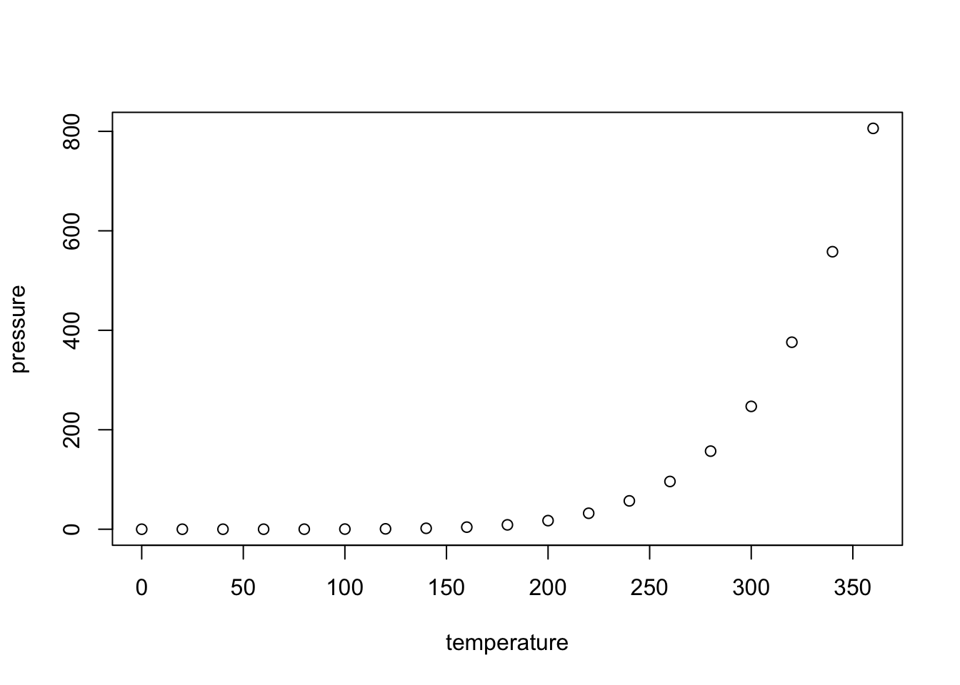  
 Max.   :360   Max.   :806.0000  

Including Plots

You can also embed plots. For example, here’s a plot of pressure vs temperature:

pressure-plot

plot(pressure)

Insert this code at the begining of rmarkdown file.

options(repos = c(CRAN = "https://cran.rstudio.com/"))
knitr::opts_chunk$set(message = FALSE)

5.0.7 Chunk options

The most important set of options controls if your code block is executed and what results are inserted in the finished report:

• eval = FALSE prevents code from being evaluated. (And obviously if the code is not run, no results will be generated). This is useful for displaying example code, or for disabling a large block of code without commenting each line.

• include = FALSE runs the code, but doesn’t show the code or results in the final document. Use this for setup code that you don’t want cluttering your report.

• echo = FALSE prevents code, but not the results from appearing in the finished file. Use this when writing reports aimed at people who don’t want to see the underlying R code.

• message = FALSE or warning = FALSE prevents messages or warnings from appearing in the finished file.

• error = TRUE causes the render to continue even if code returns an error.

Option	Run code	Show code	Output	Plots	Messages	Warnings
eval = FALSE
include = FALSE	✓
echo = FALSE	✓		✓	✓	✓	✓
results = "hide"	✓	✓		✓	✓	✓
fig.show = "hide"	✓	✓	✓		✓	✓
message = FALSE	✓	✓	✓	✓		✓
warning = FALSE	✓	✓	✓	✓	✓

5.0.8 PDF Reports: Install tinytex package

• To create PDF documents from R Markdown, you will need to have a LaTeX distribution installed. Although there are several traditional options, I recommend that R Markdown users install tinyteX.

Install tinytex package

tinytex::install_tinytex(force = TRUE)

To learn more about R Markdown, Check this ebook

---